 |
www.chameleongroup.org.uk - online publication
This paper introduces the reader to the concept of virtual pitch and in particular to the model developed by Hofmann-Engl which not only extracts roots of a chord but estimates also its degree of consonance/dissonance (sonance). Hereby, the author evaluates Hofmann-Engl's approach as well as his experiments. Concluding that the models appear to be functional, they are subsequently used analyzing three pieces taken from the 20th century repertoire. Here, it becomes apparent that the models are very powerful tools uncovering structural elements of these pieces, which without the application of the models would have been impossible to detect.
Without doubt, contemporary music has been facing a great many challenges since the beginning of the 20th century, and arguably, the understanding of harmonic structure might be seen as one of its greatest. This is, while a composer operating within the framework of the major/minor tonality had been able to understand not only the internal structure of an isolated chord (such as its root and its inversions) but also its functionality in a given context (such as the relationship between the tonic and the dominant), contemporary composers working outside of this framework have no access to such knowledge. The only significant attempt to address this issue during the first half of the 20th century was undertaken by Hindemith (1937) with his Unterweisung im Tonsatz. Here, Hindemith endeavored to classify chords and to reestablish a new harmony theory. However, Hindemith's approach was soon exposed as being pseudo-scientific and in fundamental assumptions wrong (compare Cazden, 1954). During the next few decades, so it appears, the notion of a new approach to harmony had died and contemporary composers seem to have followed either their own system or their intuition.
During the seventies, Terhardt published a series of articles on virtual pitch (e.g. 1977, 1978) culminating in his article Calculating virtual pitch (1979), where he applied the concept of virtual pitch to musical analysis. The concept of virtual pitch is based upon the discovery of residual pitch by Schouten (1940), where residual pitch refers to the human ability to hear the first partial tone of a harmonic sound even if the first partial tone is not present within the spectrum of the sound (for a detailed introduction see Moore, 1997). Terhardt's basic assumption is, that a complex harmonic sound will be scanned by an internal mental processor searching for the virtual pitch which represents the spectrum best. Unlike residual pitch a virtual pitch is a pitch which might not be heard but which is implied and which, in some sense corresponds to the root of a chord. However, Terhardt's model soon found itself under scrutiny. This is, although Terhardt's model predicts the root of a major chord in accordance with traditional music theory, it differs when applied to a minor chord (i.e. the minor chord: a - c - e produces, according to Terhardt, the root d). This discrepancy prompted Parncutt (1988) to modify Terhardt's model by introducing a kind of minor third subharmonic (not dissimilar to Hindemith's approach), thus obtaining the root as traditionally ascribed to a minor chord. However, as Balsach (1997) points out, Parncutt's approach itself leads ultimately to contradictions. Moreover, Balsach offers a stringent argument that a is not the root to the a-minor chord, as a-minor can not serve as the dominant to the d-major/minor chord. Balsach discusses also which partial tone ought to be the cut-off point, dismissing both Terhardt's cut-off point (9th partial tone) and Leman's (1995) cut-off point at the 15th partial tone. However, as we will see, Balsach's cut-off point (7th partial tone) renders his approach unable to explain a series of data. Leman amongst others used also inversely proportional weights for each partial tone. However, as argued by Hofmann-Engl (1990), the weights as set by these researchers lead also to discrepancies between measured and predicted data. To complicate matters, there are two common explanations for the phenomenon of virtual pitch, one of which is called the pattern recognition model and the other the temporal model. Terhardt's approach belongs to the first class and Schouten's approach belongs to the second class (compare Moore, 1997). The discussion, which of these approaches is most successful, is as yet unresolved. However, as shown by Wightman (1973), the "peak-picker" approach can not explain the pitch perception of an inverted signal which produces the same pitch perception as the non-inverted signal. Although Meddis & Hewitt (1991) developed an improved version of a temporal model which is in agreement with Wightman's results, their model does not, as admitted by these researchers, resolve a series of other problems. At the same time pattern recognition models face the problem that they are generally phase shift insensitive. True that naturally produced sounds, such as a chord played on a piano, are phase shift insensitive (compare Moore, 1997), but the perception of a quasi frequency modulated stimulus is phase shift sensitive (Ritsma & Engel, 1964). As this article will deal with musical sounds, the issue of phase shift sensitivity will be of no relevance.
As the reader might conclude by now, there exists great diversity and confusion about the concept of virtual pitch, and it does not surprise that there have been few attempts to make use of this concept to establish a theory of contemporary harmony. However, the author decided to consider Hofmann-Engl's approach (1990, 1999) for three reasons. Firstly, Hofmann-Engl delivered reasonable experimental support for his model when applied to musical chords, secondly it includes an algorithm estimating sonance (degree of consonance/dissonance) of a chord and thirdly, he demonstrated that his model can be a powerful tool for producing compositions outside the major/minor tonality. Thus, the author will introduce this model, discuss the experimental evidence and finally show how the model is suitable for the analysis of contemporary music referring to three stylistically different compositions.
As mentioned above, there exists disagreement on how many partials should be considered for the implementation within a virtual pitch model. While Terhardt considered the 9th partial to be the cut-off point, Leman's cut-off point coincided with the 15th partial and so did Hofmann-Engl's. The argument given is that after the 15th partial intervals become unspecific. That is, they could belong to so many different subharmonics of similar quality that they can be neglected. This assumption appears to be in contrast to the findings by Houtsma & Smurzynski (1990) whose results indicate that higher partials which cannot be discriminated individually can still produce a pitch sensation (implying that audibility of single partials and the perception of virtual pitch are not to be equated). Still, if we take into account that Hofmann-Engl's virtual pitch model serves to extract roots of chords and is applied to the 12-tone scale, the decision to take the major seventh as the cut-off point seems sensible. Moreover, as we will see, this decision is supported by the experimental data. Additionally, setting the cut-off point as low as the 9th partial leaves a major seventh chord (e.g., c - e - g - b) unexplained. Interestingly, even Rameau (1722) includes the major seventh and ninth as intervals supporting a fundamental bass. Thus, following the argument above, the virtual tone (or root) c is supported by the tones c, g, e, bb, d and b. Generally speaking: A virtual pitch is supported by the tones a fifth above, a major third above, a minor seventh above, a major second above and a major seventh above the root. Note, the 11th and 13th partials are not included within this model, as they would produce roots outside the well tempered 12-tone chromatic scale. However, if working with other tuning systems (e.g. microtone scale), the 11th and 13th partial will have to be considered.
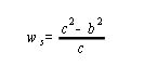
Balsach (1997) argued that the weights as set by various researchers are set arbitrarily and inversely proportional to the order they appear in the overtone series. Balsach is correct in stating that these weights are set arbitrarily. However, the following argument by Hofmann-Engl (1990) makes clear that weights will be necessary:
As observed by Stumpf (1965) two simultaneously played tones display a tendency, dependent on interval size, to be judged as one. Generally the octave is most likely to be judged to be one tone followed in decreasing order by the fifth, the forth, the minor/major third, the minor seventh and the tritone. Now, if the octave has a stronger tendency to produce a single pitch sensation than the minor seventh, we can infer that the octave supports one virtual pitch more than does the minor seventh. Hence, weights will be necessary.
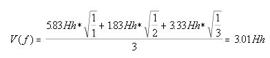
The question of how to set these weights received some attention in Hofmann-Engl these (1990). During some pre-experiments, he rejected weights to be set inversely proportional as well as an exponential approximation of Stumpf's Verschmelzungsgrad (degree of fusion). Instead he approximated the mean order of each interval as it appears first within the overtone series (e.g. the mean order of the octave is: (1+2)/2 = 1.5 while the mean order of the fifth is (2+3)/2 = 2.5). For the purpose of approximation, he used a polynomial and reported the following formula to be suitable:
|
The next step is not dissimilar when compared to other virtual pitch models (compare Terhardt 1979): In order to extract the root of a given chord, the six subharmonics of each tone of the chord are listed. We take the c-major chord in root position as an example (table 1):
| weight | c (tone 1) | e (tone 2) | g (tone 3) |
| 6.00 Hh | c | e | g |
| 5.83 Hh | f | a | c |
| 5.33 Hh | g# | c | d# |
| 4.50 Hh | d | f# | a |
| 3.33 Hh | a# | d | f |
| 1.83 Hh | c# | f | g# |
Additionally to these weights, so argues Hofmann-Engl (1990) further, a lower tone ought to be weighted more than a higher tone. This approach is supported by Terhardt, Stoll & Seewann (1982a, 1982b) who found that inverting a chord alters the perception of the virtual pitch indeed. Additionally, the music theorist might be reminded that a tonic chord in its first or second inversion is unlikely to be accepted as the concluding chord to a composition (e.g. the chord e - c - e - g). This is, should the root of a tonic chord be also its lowest note, we will find that the tonic note will also be the strongest virtual pitch. Applied to our example, the decision will be made that the subharmonics as produced by the tone c will have to be weighted more than the subharmonics of the e, which itself will receive higher weighting than the tone g and so on. The exact weight used by Hofmann-Engl is:
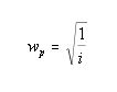 |
where wp is the weight according to the position of the tone i within the chord. For the lowest tone i = 1, for the next higher tone i = 2 etc..
Finally, the strength of a specific virtual tone (root) is calculated as the mean strength of all subharmonics supporting this root (in case a tone of the chord does not support this root it enters the equation with the value 0). The formula is:
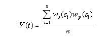 |
where V(t) is the strength of the virtual tone t, ws(si) the spectral weight of the ith subharmonic of the chord, wp(si) the weight of the ith subharmonic according to the position of the tone within the chord, n the number of tones the chord consists of and the constant c = 6 Hh
Applying this formula to the c-major chord in root position, we obtain for the root (virtual pitch)c:
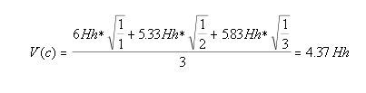
and for the root f:
We list below all the virtual pitches which are implied by the c-major chord (table 2):
| Chord: c-major (root position) | |||||||||||
| virtuality of c is 4.37 Hh | virtuality of g is 1.15 Hh |
| virtuality of f is 3.01 Hh | virtuality of a# is 1.11 Hh |
| virtuality of d is 2.28 Hh | virtuality of f# is 1.06 Hh |
| virtuality of a is 2.24 Hh | virtuality of d# is 1.02 Hh |
| virtuality of g# is 2.13 Hh | virtuality of c# is 0.61 Hh |
| virtuality of e is 1.41 Hh | - |
As we find, the root c fetches the strongest virtuality, followed by the root f, the root d and so on. This is, just as it is the case with other virtual pitch models, a chord fetches not only one root, but a number of roots of varying strength. Hofmann-Engl interprets this in a probabilistic fashion. This is, the probability for a listener to hear c as the root of the c-major chord is higher than the probability to hear f as its root. The following three audio examples may help to illustrate this:
In the first example, we hear the c-major chord first followed by the bass note c, while in the second example, we hear the c-major chord first followed by the bass note f. The third example is identical with the first and second except that we now hear the bass note d. Clearly, while c fuses with the chord well, f fuses less well but still better than d. Even within the framework of traditional harmony, these results are sensible: c is the strongest root (c-major chord), but f fetches still high virtuality (3.01 Hh). This is, the triad c - e - g together with f as its bass note is a f-major major-7th chord. In contrast to this, the root d fetches low virtuality and can not function as a bass note to the c-major triad.
The model is particularly interesting if we consider the a-minor chord. The data are listed in table 3:
| Chord: a-minor (root position) | |||||||||||
| virtuality of d is 3.64 Hh | virtuality of ab is 1.25 Hh |
| virtuality of f is 3.50 Hh | virtuality of e is 1.15 Hh |
| virtuality of a is 3.12 Hh | virtuality of g is 1.11 Hh |
| virtuality of c is 2.44 Hh | virtuality of f# is 0.86 Hh |
| virtuality of b is 1.50 Hh | virtuality of c# is 0.43 Hh |
| virtuality of bb is 1.39 Hh | - |
At first, it appears that these results contradict with traditional harmony theory just the same as Terhardt's model did. This is, both models do not identify a as the strongest root of the a-minor chord. However, scrutinizing the data for the a-minor chord in detail, we find that d has the highest virtuality and yet at the same time the virtuality of f is smaller by only 4%. The traditional root a itself fetches a virtuality only 14% less than the virtuality of the root f. Indeed, we find that the a-minor triad is ambiguous even within classical theory. Adding the bass note a to the a-minor chord causes a to fetch the highest virtuality, adding the bass note f to it, we obtain the f-major major-7th chord and adding the bass note d to it generates the d-major minor-7th major-9th chord with omitted third. The ambiguity of the a-minor chord is well reflected within this model. The only question which might disturb the reader is, whether the a-minor chord fuses better with f and d than it does with a. The author argues that this is the case indeed and hence Parncutt's model appears to be at fault as does Leman's by weighting the partials inversely proportional to their order (where a becomes the strongest root). The reader might also recall the argument as stated above; according to Balsach an a-minor chord does not fetch the root a, otherwise it could function as the dominant to d-major/minor which it does not. Still, the reader might argue that almost all pieces in a minor key end in the tonic minor, hence - so the argument - the minor chord does support the traditional root. Granted, that often enough this is true, but just by adding the bass note a to the a-minor chord, will ensure that - according to Hofmann-Engl's model - a is the strongest virtual pitch indeed. Finally, we might also consider that Baroque composers quite frequently ended a minor composition with the tonic major chord. The same is not true for major composition, which always end on the tonic major chord (at least the author is not aware of one single such composition). However, the reader might judge for her/himself by listening to the following three audio samples:
The small difference between f and d appears to the author to be very clear. Thus, the author claims, the model does not conflict with traditional harmony theory. However, the strength of the model becomes only apparent when applied to non-traditional chords. We will consider two of these chords. The first one is the cluster triad bb - b - c and the second the Webern triad (compare Hofmann-Engl, 1999) c - c# - f#. The cluster triad fetches c as the root with the strongest virtuality (3.08 Hh) followed by bb (2.64 Hh) with a difference of 14%. For the Webern triad we obtain d as the strongest root (2.95 Hh) followed by g# (2.64 Hh), a difference of 11%. The two audio samples below might help to illustrate how the roots with the highest virtuality match the cluster and the Webern triad:
Using both, either Terhardt's or Balsach's model cannot explain both of these triads. Further, a more advanced "peak picker" model (Meddis & Hewitt, 1991) identifies the b as the strongest root for the cluster triad and the quarter tone above c# for the Webern triad. While it appears to the author unlikely that b will be the dominant root for the cluster triad (it fetches a virtuality 35% lower than the root c), a quarter tone might even be somewhat correct but forces us outside the 12 tone scale. It seems to the author that Hofmann-Engl's model makes a strong case even before we consider the experimental data, which will provide further evidence. However, we briefly will describe the algorithm predicting the consonance/dissonance degree of chords (called sonance) first.
While Hofmann-Engl's virtual pitch model (1990) or better say root extraction algorithm is fairly well described, there is a serious lack of discussion within the section of his sonance algorithm. Even the formula he delivers remains largely unexplained, so much so that it could easily be dismissed if the experimental data he provided had not deliver good support for it. He reasons that many computer simulations and preliminary experiments generated the formula and that it would be tedious to examine each step.
Consonance and dissonance are concepts that have been interpreted in various ways (compare Eberlein, 1994), none of which seem very convincing. Hofmann-Engl's approach appears to be closest to Husmann's (1953) basic assumption. Husmann maintained that a sound (chord) will be perceived the more discordant the less clear the harmonic spectrum is. This is, two tones, where many partials coincide, a higher degree of consonance is to be expected. However, as shown by Eberlein (1990), this does not seem to be the case. Hofmann-Engl agrees with Husmann, but relates the virtual pitch spectrum to the degree of consonance rather than to the partials. His basic hypothesis is:
A chord produces a set of virtual pitches. The simpler this set of the virtual pitches is, the more consonant it will be. This is, the higher is the sonance value.
This statement has to be understood in the following manner: Should a chord generate a great deal of different virtual pitches, this will contribute to making this chord complex. The simplest chord we could have, would produce just 6 virtual pitches and the most complex chord 12 different virtual pitches (note, this model as it stands applies to the 12-tone chromatic well tempered tuning system only). A second factor, which is of even greater importance, is, according to Hofmann-Engl, the strength of the strongest virtual pitch compared to the other virtual pitches. Clearly, should the strongest virtual pitch be sufficiently stronger than the others, a listener could be expected to pick this strongest virtual pitch with ease as the one which represents the chord. On the other hand, should the strongest virtual pitch be close to the others in terms of its strength, a listener might be more confused about which virtual pitch to pick. The more ambivalent the chord is, the more complex it is, and the less ambivalent it is, the simpler it is. The exact formula, as given by Hofmann-Engl, is:
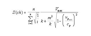 |
where S(ch) is the sonance (with unit Sh = Schouten) of the chord ch, vmax is the virtuality of the strongest root, k = 6 Hh/Sh, m is the number of virtual pitches produced by the chord ch, vpmax is the virtuality of the strongest root in percent (= vmax divided by the sum of all virtual pitches of the chord ch), c = 0.223 (the maximal limit the strongest root can fetch), n the number of tones the chord ch consists of and i the ith tone of the chord ch.
The term:
 |
neutralizes the weight as attached to the virtual pitch according to the position of the tone within a given chord. This is, chords consisting of only octaves will fetch maximal sonance (=1 Sh). The decision to rate all octaves as sonant as single tones appears problematic especially when we consider that the degree of fusion (Verschmelzungsgrad) for octaves lies around 75%, hence they can be perceived as being different to a single note. It appears that Hofmann-Engl's wish to classify all octave chords into one group is driven by the understanding of a composer who sees octaves as nothing more than increasing the volume of a single tone. But it appears to the author that this decision will limit the validity of the algorithm to some extend. As we will see later Hofmann-Engl's experimental data do not address this issue.
The term vmax correlates sonance to the strength of the dominant root. This part of the equation is not dissimilar to Terhardt's approach (1976). However, the inversely correlated component of the equation is more complex. The square root term has the format of a relativistic correction term. This is, the smaller vpmax the more will m (the number of virtual pitches produced by the chord ch) be taken into account. If we consider a single tone (or octave chords), we obtain vpmax = cp rendering the square root 0 and eliminating m2/k. Thus we obtain, S(octave chord) = 6/6 Sh = 1 Sh. Summarizing we can say that Hofmann-Engl considers three factors which influence sonance:
In order to demonstrate how the algorithm works, we will calculate the sonance for the c-major chord c - e - g:
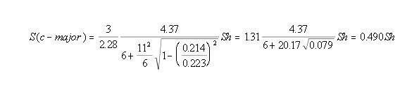
For the minor chord we obtain: S(minor) = 0.294 Sh, for the Cluster Triad: S(Cluster Triad) = 0.171 Sh and for the Webern Triad: S(Webern Triad) = 0.160 Sh. It appears that the Webern triad is slightly more discordant than the Cluster triad and both are more than 40% more discordant than the minor chord while the major chord is the most consonant triad of all. This makes intuitively sense. The experimental data below are in agreement with this. However, before we consider the data, it is important to discuss another two issues: Firstly, the algorithms, as they stand, are sensitive towards inversion. This is, a chord in root position can fetch a different dominant root and also a slightly different sonance. This is true for the minor chord. For instance a-minor root fetches d as the dominant root while the a-minor chord in second inversion fetches the dominant root a. Admitted, the a beats the d by less than 1%, but that inversion should effect the root seems again to be in conflict with traditional harmony theory, although, as mentioned above, it is in agreement with some experimental data (Terhardt, Stoll, & Seewann, 1982b). Hofmann-Engl did not address this issue theoretically nor did his experiment investigate it. However, we might argue that we find a triad most commonly in conjunction with a bass note. Inverting a major/minor triad while keeping the same bass note does not alter the dominant root. Yet, changing the bass note let us say of a c-major chord to the third e will alter the perception of the chord enough to disable the chord from functioning as the concluding chord of a piece written in c-major. Hence, the author concludes not to dismiss Hofmann-Engl's model until there exits evidence against it. The second and final issue has to do with the fact that Hofmann-Engl himself offered some critique which effects the reliability of the model. Factors which are mentioned are the fact that pitch is treated in pitch class sets rather than absolute pitch, timbre is not included in the algorithm and neither is loudness. Hofmann-Engl stressed that the algorithm might at times produce wrong results but he maintained that it can be an approximating tool facilitating the work of a composer as well as the work of a musicologist.
Measuring virtual pitch in an experiment is somewhat difficult. It appears to the author that neither Terhardt's method (1977), where participants were asked to notate the implied sequence of roots for a sequence of chords, nor the method employed Schulte, Knief, Seither-Preisler & Pantev (2000) where participants were asked to listen to a series of complex tones which implied the melody "'Frere Jacques" until they recognized the tune after several days of training, is sufficient. As we will see, Hofmann-Engl's approach has some advantages but does not come without some serious problems. He decided to play a chord A followed and played simultaneously by a bass note e. After an interval of ca. 2 sec, he played a chord B followed again by the bass note e. Participants of his experiments were asked to state which of the chords would fit the bass note best by either ticking chord A or chord B. The chords used are listed in table 4:
| Trial Number | Chord A | Chord B |
| 1 | e - a - c# - e | e - g# - b - e |
| 2 | e - g - a# - e | e - b - c# - e |
| 3 | e - g# - d# - e | e - g - b - e |
| 4 | e - f - c - e | e - f# - c - e |
| 5 | e - f - d - e | e - c# - d - e |
| 6 | e - g - g# - e | e - a - a# - e |
| 7 | e - a# - d - e | e - f# - a - e |
| 8 | e - g - d# - e | e - f - g# - e |
| 9 | e - f - b - e | e - f# - g - e |
| 10 | e - a# - c - e | e - f# - g# - e |
As we can see all "corner-notes" are e-s. This is, so Hofmann-Engl, to avoid melodic interference. However, this poses a substantial restriction on the set of available chords and thus, limits the validity of the data. There are a number of other minor issues which diminish the quality of Hofmann-Engl's experiment: the trials were not randomized and they were not played in both orders A - B and B - A. Hence some of the results obtained might be biased due to context effects. Still the most significant shortcoming is the following: while it is clear that familiarity does not imply preference under specific conditions (Berlyne, 1970), it is generally accepted that familiarity implies preference indeed (Newcomb, 1961). Comparing a stimulus, which is familiar, with a stimulus, which is novel, will generally lead to a preference of the familiar stimulus. The author run a small test involving 8 participants (age range 7 to 63), who were ignorant of music theoretical issues, asking them which of two chords they preferred, a c-major chord or a Webern triad. All participants preferred the c-major chord over the Webern triad. The probability for this to be chance is p < 0.005. The question Hofmann-Engl asked the participants in his experiment: "Which chord fits the bass note best", implies the question which chord the participants preferred and hence a bias can be expected if a familiar stimulus is compared to a novel stimulus. Surprising maybe to Hofmann-Engl, but this is exactly what happened during his experiment. Trial 2 compared a diminished chord to a non-traditional chord. Participants (all in all 73), showed a small preference (3 more "votes") for the diminished chord, although the algorithm predicts a preference for the non-traditional chord. Trial 3 compared a minor chord to a non-traditional chord, and now there is even stronger preference (38 more "votes") for the minor chord. Finally trial 7 compared a minor minor-7th chord to a non-traditional chord. This time, the algorithm predicts that a substantial preference for the non-traditional chord ought to be observed but only a small preference (2 more "votes") was observed. Had it been the intention to compare familiar with novel stimuli, it would have been necessary to ensure that participants are sufficiently familiarized until the familiarity effect had been eliminated. However, there is a chance that even familiarization would not suffice because listeners are constantly exposed to major/minor tonality. Hence trials involving the comparison of a familiar with a novel chord will have to be excluded. We are now left with 7 trials. Hofmann-Engl's assumption now is the following: The greater the difference is between the virtualities of chord A and chord B, the stronger is the difference in preference. This is, the larger is the number of participants who favor the chord with the stronger virtuality. This number then is given in percentage (e.g. if 75 participants preferred chord A and 25 participants chord B a difference of (75-25)/100 = 50% would be computed). The following table (table 5) lists the predicted differences and the measured differences:
| Trial | Predicted difference | Measured difference |
| 1 | 44% | 62% |
| 4 | 20% | 33% |
| 5 | 0% | 11% |
| 6 | 25% | 23% |
| 8 | 16% | 3% |
| 9 | 8% | 23% |
| 10 | 37% | 62% |
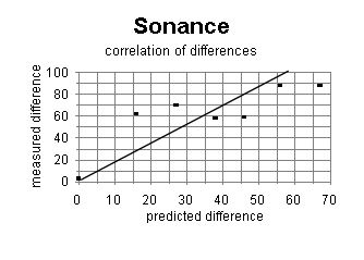
The correlation of these trials is: r2 = 0.67 with p < 0.03. The graph below illustrates this correlation.
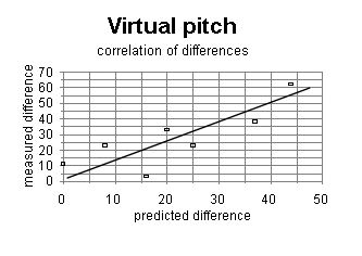
where the predicted difference is calculated as: (V(chord A) - V(chord B) )/V(chord A) for V(chord A) > V(chord B) and (V(chord B) - V(chord A) )/ V(chord B) for V(chord B) > V(chord A) and the measured difference as: ABSOLUTE (people preferring chord A - people preferring chord B )/all participants.
The author concludes that Hofmann-Engl's evidence on virtual pitch is reasonably convincing even if it does not allow for the comparison of familiar with novel chords. We now will consider his data in respect to sonance.
The measurement of sonance is, according to Hofmann-Engl, a straight forward task: Chord A is to be compared with chord B where we expect that the larger the sonance difference between the two chords, the more participants will identify the more discordant chord correctly. The differences are calculated in the same manner as before. This is, should 75 participant identify chord A as being more discordant and 25 participants chord B, we would obtain the difference: (75-25)/100 = 50% ). However, after conducting the experiment, Hofmann-Engl admits that one trial (out of 8 trials) was in contrast to the prediction due to context. However, if context can influence ratings, then Hofmann-Engl would have to admit that testing sonance is not as straight forward as he professed to proclaim. The author will list the chords, the predicted and measured data in table 6:
| Trial | Chord A | Chord B | predicted difference | measured difference |
| 1 | g - c - e | f - f# - e | 67% | 88% |
| 2 | g# = a# - e | g - a# - e | 38% | 58% |
| 3 | f# - c# - e | c# - d - e | 56% | 88% |
| 4 | f - d - e | f# - a - e | 27% | 70% |
| 5 | c - d# - e | a# - d# - e | 0% | 3% |
| 6 | f - a - e | g# - c - e | 7% | -41% |
| 7 | f# - b - e | b - d# - e | 16% | 62% |
| 8 | a - d - e | f - a# - e | 46% | 59% |
It appears that the sonance algorithm is fairly powerful. Even without excluding trial 6, we obtain r2 = 0.62 (p < 0.02). However, excepting that trial 6 is wrongly predicted due to context (for a detailed explanation compare Hofmann-Engl, 1990), we obtain: r2 = 0.70 (p < 0.02). The graph below illustrates this.
where the predicted difference is calculated as: (S(chord A) - S(chord B) )/S(chord A) for S(chord A) > S(chord B) and (S(chord B) - S(chord A) )/ S(chord B) for S(chord B) > S(chord A) and the measured difference as: ABSOLUTE (people rating chord A as more dissonant - people rating chord B as more dissonant)/all participants.
The author concludes that the experimental data as given by Hofmann-Engl indicate that both the virtual pitch and the sonance algorithm are operational. It is also apparent that their reliability is limited. Hofmann-Engl (1990) discusses some of these limitations. Firstly, timbre is not included and yet clearly a tone with a sharply defined pitch will be of greater significance than a tone less well defined. Secondly, loudness is not included and yet again a louder tone will be of greater importance than a softer tone. Thirdly, the pitch range within which this algorithm is valid has not been discussed. Fourthly, Hofmann-Engl (1990) observed that expertise is a factor affecting experimental measurements (again not covered by the algorithm), and finally, the issue of context and cultural factors is touched only briefly without him being able to come to some sort of systematic conclusion. Thus, it is clear that the algorithms are limited in their reliability. How limited this reliability is, is an issue for further experimentation, which this article wishes to encourage. Hofmann-Engl (1999) has demonstrated that the algorithms can be utilized within contemporary composing involving virtual tonality and virtual modulation. The author will now demonstrate how the algorithms can be used to analyze three examples of 20th century music. This is not in order to show that the algorithms as they stand present a final answer, but to illustrate that virtual pitch and pitch salience (sonance) can be of great help analyzing contemporary music.
This small piece for piano has been subject of analysis, but, as Phleps (2001) remarked, none of which have been satisfying. Phleps's own analysis is interesting but leaves the question of the cognitive structure of the piece untouched.
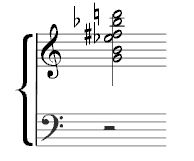
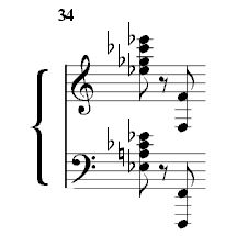
In order to the cognitive structure in terms of virtual pitch, the author examined the final chord of the piece (g - b - eb - f# - bb - d) first. The dominant root is g with 2.17 Hh (figure 1).
|
Figure 1 |
|
Figure 2 |
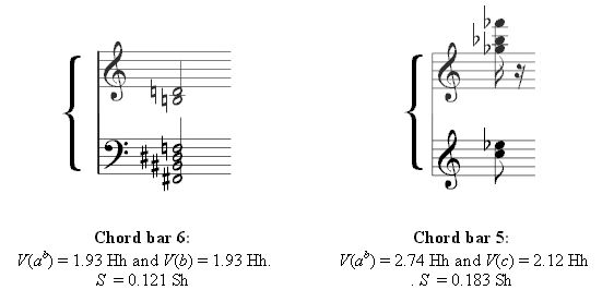
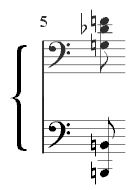
Although the piece is centered around g, there exists a conflict with the center ab. This conflict is confirmed if we extract the root from the chord in bar 6 (3rd quarter beat). The dominant root is ab and b (both fetching 1.93 Hh). The strength of the center ab receives further support when extracting the root of the chord in bar 5 (1st quarter beat). The center ab is clearly the strongest root with V(g) = 2.74 Hh followed by c with V(c) = 2.12 Hh (figure 3).
|
Figure 3 |
It is also interesting to note that, while the major/minor tonality derives the dialectical conflict from the conflict between the tonic and dominant, Schoenberg's composition derives this conflict from two tonal centers a minor second apart from each other, or - in more classical terms - between the tonic and the leading note, while the leading note maintains preeminence. In this sense, Schoenberg adheres to an underlying classical concept of a dialectical conflict but breaks radically loose from classical tradition by shifting this conflict into a dimension unthinkable within classical tradition. This result is also interesting when compared to traditional harmonic analysis (compare Kopfermann, 1980) which identifies the piece centered around G major due to the continuous repetition of the interval g - b, and where the first melody phrase in bar 2 and three is seen as a conflict between tonic and dominant. The chord in bar 5 is identified as being some form of diminished subdominant, the chord in bar 6 as form median chord and the final chord as a distorted tonic. However, such an analysis fails to describe the chords appropriately. It fails also to uncover the appropriate harmonic conflict.
Admitted, this analysis is brief, but the author maintains that this analysis enabled us to uncover the basic harmonic structure of the piece in terms of virtual pitch.
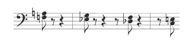
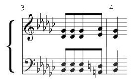
Bartok's piece - similar to Schoenberg - builds upon two tonal centers. This time, the conflict is between the center eb and ab, where eb is the dominant center. The key signature indicates that the piece is either in gb-major or eb-minor. Considering that eb is the central tone, we assume that the piece is close to eb-minor.
The opening phrase (bar 1 to 4) commences and closes with the chord: bb - eb - db - gb. The dominant root is eb with V(eb) = 3.16 Hh. This phrase is repeated in bar 5 to 8 almost identically with the opening (4 + 4 = 8 bar phrase (!) ). The root sequence of these two phrases is: eb - e - eb - gb - eb - d - eb. This indicates that the tonality of eb-minor is undermined by the appearance of a chord with root e. The last chord in bar 3 (a - d - eb - gb) produces the strongest root d with a sonance of S = 0.143 Sh while the first chord in bar 4 (bb - eb - db - gb fetches a higher sonance with S = 0.208 Sh (fig. 4).
|
Figure 4 |
This form of "cadence" is close to a classical cadence in as much as a discordant chord is resolved into a more concordant chord (in contrast to Schoenberg). The root d functions as the leading note to the root eb.
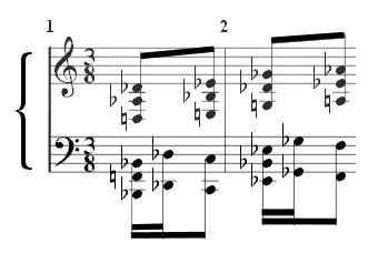
The next eight bars end with the same "cadence" on eb. However, each of the last quarter beats of bar 9 to 14 fetches the chord: g - c - eb - ab with the dominant root ab (V(ab) = 2.99 Hh). The root sequence itself is persuasive to be regard ab as the central root of this passage: bb - b - c - ab - bb - b - c - ab - d - ab - d - ab - bb - b - c - ab - bb - b - c - ab (bar 9 to bar 14). In common with phrase 1 (bar 1 to bar 8), this phrase is modeled according to the schema of the classical period: 4 bars semi-close (comparable to an imperfect cadence) 4 bars close (comparable to a perfect cadence).
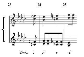
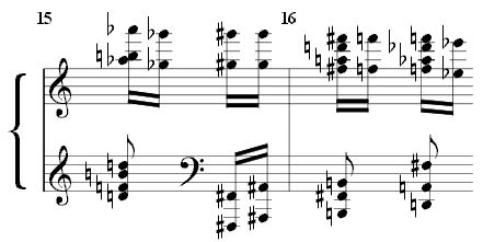
The next phrase breaks away from the classical model in more than one way. Firstly, it runs from bar 17 to bar 30 comprising 14 bars in all and secondly, it consists of three overlapping sections. The first section (bar 17 to 20) features only four chords within bars 17 to 18, all of which consist of the notes: bb - eb - db - gb with dominant root eb (V(eb) = 3.16 Hh). Bar 19 effects a shift from the center eb to b for two bars. This shift to b is the only such shift throughout the piece and hence is only of local importance as a response to the two previous bars. Bar 23 to bar 24 illustrates the overlap of pattern 2 leading to the chord bb - eb - db - gb with dominant root eb in bar 25. In fact, from bar 24 to bar 30, the root sequence is f - gb - e - eb (figure 5), which is repeated four times.
|
Figure 5 |
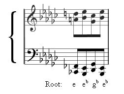
However, the last time the pattern is repeated it breaks up on the root e instead of the root eb. The point, that an interrupted ending is intended is confirmed by the fact that the sequence breaks on an up-beat followed by a rest and a new bar-wise harmonic and rhythmic pattern in bar 31 to 34 (figure 6).
|
Figure 6 |
Here, we find chord eb - ab - gb - cb used 8 times, confirming that ab is a contrasting central root to eb indeed. The following section (bar 35 to the end) is of particular harmonic interest in as much as it appears to function as the coda to the piece. The composition finishes on the octave eb - eb. The penultimate chord is: f - bb - ab - db which fetches the dominant root gb. Maybe not by chance, the relationship between eb and gb is manifested by the fact that eb-minor is the relative key to gb-major.
Now, bar 35 to bar 40 contains three times the pattern: broken chord - concluding chord. Each time the concluding chord fetches the dominant root gb (the root which leads to the conclusion of the piece). The root sequence is: c - gb - g - gb - c - gb, involving the tritone and the minor second - both intervals of significance for the 20th century (Fucks & Lauter, 1965). Bar 41 to bar 42 anticipates the ending of the composition by making use of unison octaves ending on the contrasting central root ab.
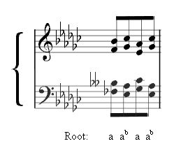
The following passage (bar 43 to 45) is a reminiscence of bar 31 to 34. However, instead of the contrasting central root ab, the pattern represents now the central root eb (figure 7).
|
Figure 7 |
Interestingly, this pattern contains the root gb followed by the root eb, again anticipating the ending. The final section 47 to bar 50 fetches the root eb for the bars 47 to 49 with the last eights beat in bar 49 on the root gb and the concluding octave on eb at the very end.
Unlike the Schoenberg example, Bartok does not create so much a conflict between the two central roots, but utilizes them in order to establish contrast. The author concludes that by applying the virtual pitch model, as described above, we obtain not only a consistent harmonic analysis of the piece, but gain some important insight into the cognitive structure of the composition. Note, we did not apply the sonance model to Bartok's composition because, due to the fact that all chords are composed of fourths, they catch a similar sonance value. This means, that Bartok's piece is harmonically static in as much as the level of consonance/dissonance is varied only slightly throughout the piece and cannot be regarded as being of significance to the piece.
Szymanowski's Etude is constructed by using bass octaves which often appear with an additional fifth (e.g. bb - f - bb). Hence, in many cases the dominant root coincides with the bass octaves. However, this is not always the case for instance in bar 5 (figure 8) where the bass b fetches the dominant root g.
|
Figure 8 |
Szymanowski's approach to sonance is traditional in as much as "cadence-sections" are resolved into chords of relative high sonance. This is true for chord bar 7 (eb - eb - f - f) S = 0.38 Sh, chord bar 13 (ab - ab - db - db) S = 0.678 Sh, chord bar 18 (d# - a - d# - f# - b - f#) S = 0.317 Sh, chord bar 23 (f - f - a - c - eb - a) S = 0.378 Sh, chord bar 34 (eb - a - cb - eb - gb - cb - eb) S = 0.318 Sh and the last chord (f - f - f - f) S = 1 Sh. The sonance of all other chords lies around the value S = 0.25 Sh (range: 0.16 Sh to 0.29 Sh).
The composition opens with the root bb and comes to a conclusion on the root f. In fact, both roots are the most common roots throughout the entire piece with f re-occurring 21 times and bb 17 times (scanning the piece in eights beats). The root with the next highest reoccurrence is g with 9 re-occurrence. The first cadence (bar 7) fetches f as the dominant root, the second cadence (bar 13) fetches db, the cadence in bar 18 fetches b, in bar 23 it is f again, in bar 34 it is b and the final unison octaves fetch the root f. While the root f is of cadencial importance 3 times, bb does not once appear in such context. Hence, we consider f to be the central root of the piece. The root bb neither creates a dialectic conflict nor a contrast. The use of bb functions, as we will see, to hide the importance of the tritone within this composition.
The underlying pattern for the root sequences appears at the beginning of the piece (figure 9):
|
Figure 9 |
The roots are: bb - c - eb - f. The pattern is: major second (up or down) - larger interval - major second (up or down). This pattern dominates the composition from bar 1 to bar 10 and again from bar 24 to bar 26. This pattern appears in distorted form in the middle section of the piece (bar 14 to bar 23) not dissimilar to the elaboration of an invention. We give an example (figure 10):
|
Figure 10 |
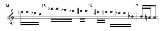
Here, the sequence of the roots is: g - f# - b - bb. While the first three roots are dominant, the root bb is not the dominant root, but d is, with V(d) = 1.99 Hh and V(bb) = 1.96 Hh. However, the difference between the roots is so small, that due to the context bb might take supremacy over the d. The reader might argue that this appears to be a dubious assumption. But even if we maintain that d is the dominant root, we obtain: g - f# - b - d, still a distortion of the original pattern. However, trying to interpret this passage simply as a distortion of the original pattern will fall short, as it leaves the main principle of this passage unexplained. In order to uncover this principle, we will have to examine the melodic lines as they appear in the soprano supported by octaves. The opening of these passages displays the following melodic pattern (figure 11):
|
Figure 11 |
This melodic line is built up by motives consisting of either two of three descending steps in minor or major seconds until the melodic line comes to an end involving larger intervals. This is true for bar 14 to 17 and bar 19 to bar 22. Bar 18 to bar 19 and bar 22 to bar 23 are cadence sections. The root structure is subordinated to the melodic structure and hence, does not display a clear pattern. However, there exists an interesting link between the descending melodic lines and the roots of the transitional passages bar 12 to bar 14 and bar 27 to bar 30: The dominant roots in bar 12 (1st beat) to bar 14 (1st beat) are: c - bb - ab - gb - f and form a descending line. The roots from bar 27 (2 beat) to bar 31 (3rd beat) are: a - g - f - b - a - a/g - g - f, which form two descending lines. It appears to the author that this is no coincidence.
The coda section (bar 31 to bar 34) reveals one more aspect which is of significance throughout the entire composition: The two final chords are (figure 12):
|
Figure 12 |
The dominant root for the penultimate chord is b with V(b) = 2.94 Hh followed by the root ab with V(ab) = 1.90 Hh (a 35% decrease in strength). There is no doubt that b is the dominant root indeed. This might at first appear to be disturbing because the final chord is f spread out over four octaves with the dominant root f. This amounts to a cadence involving a tritone progression. As mentioned above the tritone had become an important idiom within the 20th century and hence the choice to conclude a piece in this fashion might not appear to be so unexpected after all. Additionally, this tritone progression does not only appear in the final section of Szymanowski's composition, but appears within each cadence section. This is, in bar 4 to bar 5(3rd beat to first beat, root db to g), in bar 10 to 11 (3rd beat to first beat, gb to c), in bar 17 to 18 (3rd beat to first beat, f to b) and bar 23 (1st to 2nd beat, root b to f). Again, this appears to be no coincidence.
We will conclude this analysis by stating the root sequence of the coda (bar 31 to 34): bb - b/a - bb - b/a - bb - f - bb - f - bb f - f - b - f. Interestingly, there is still some uncertainty about how the piece will conclude. At first it appears that a plagal cadence might take place, only to learn at the end that the tritone celebrates superiority indeed.
This brief analysis will not be able to reveal all important aspects of the piece, but the author feels, that by referring to the concept of virtual pitch and sonance, we obtained a good insight into the overall harmonic structure of this composition by Szymanowski. Moreover, comparing the three different analysis, it seems apparent that a virtual pitch model combined with a sonance model are able to extract important and relevant elements of 20th century compositions - three compositions which are very different in style.
The author felt that - as the models are mathematically non-trivial - it seemed most appropriate to give the reader the opportunity to test the model for her/himself. The following applet application is largely self-explanatory: Keys (within the octave c to c) can be selected via mouse click and once selected, they appear marked with a red circle. A second click will de-select the key and the red circle disappears. After selecting the desired pitches, the chord can be played by pressing the play button. The data for the chord can be obtained by pressing the calculate button. The data will appear in the window below the keyboard picture ordered according to strength (the dominant root will be first followed by the second one and so on). After all virtual pitch values the sonance value appears at the end of the column. All keys can be de-selected by pressing the clear button.
The author introduced the reader to the concept of virtual pitch pointing out some issues of the current sate of research. The reader was further introduced to a specific model on virtual pitch and sonance as developed by Hofmann-Engl. The author chose this specific model as it appears to be supported by experimental data and has been shown to be a useful tool for contemporary composing. Further, the author critically reevaluated Hofmann-Engl's experimental approach and found that some of Hofmann-Engl's data are corrupt and insufficiently evaluated. However, it appeared that changes to the models were not necessary. The author finally tested the models against the background of three compositions taken from the 20th century repertoire. It was shown that the models were able to reveal the basic harmonic structure of all three pieces in a comprehensive and stringent fashion, although the three compositions in questions are very different in nature. Thus, the author concludes that these analytical examples provide further evidence that the models in questions are operational. The author decided that it would be useful to add an applet, which will allow the readers to experiment with the model themselves, at the end of this article. It is not the claim of this article that any final answer has been given in regards to the concept of virtual pitch. Rather than this, the author argues that virtual pitch is a concept which has not received sufficient interest over the last decades and that more experimental investigations, further applications to composition and to music analysis are outstanding.
The author wishes to thank R. Meddis for his valuable input to this article. Additionally, The author wishes to thank F. Hofmann for his significant improvements to the java applet.
Balsach, L. (1997). Application of Virtual Pitch Theory in Musical Analysis. Journal of New Music Research 26, 244-265
Berlyne, D. E. (1970). Novelty, complexity, and hedonic value. Perception and Psychophysics 8, 279–86
Cazden, N. (1954). Hindemith and nature, The Music Review 15.4, 288 - 306
Eberlein, R. (1990). Theorien und Experimente zur Wahrnehmung musikalischer Klänge. Europäische Hochschulschriften, 36.44
Eberlein, R. (1994). Die Enstehung der tonalen Klangsyntax. Peter Lang, Frankfurt am Main
Fucks, W. & Lauter, W. (1965). Exaktwissenschaftliche Musikanalyse. Westdeutscher Verlag, Köln
Hindemith, P. (1937). Unterweisung im Tonsatz, Schott, Mainz
Hofmann-Engl, L. (1990). Sonanz und Virtualität. MA Thesis, TU Berlin (unpublished)
Hofmann-Engl, L. (1999). Virtual Pitch and Pitch Salience in Contemporary Composing. Proceedings of the VI Brazilian Symposium on Computer Music at PUC Rio de Janeiro
Houtsma, A. J. M & Smurzynski, J. (1990). Pitch identification and discrimination for complex tones with many harmonics. J. Acoust. Soc. Am. 87, 304 - 310
Husmann, H. (1953). Vom Wesen der Konsonanz. MüllerThiergarten, Heidelberg
Kopfermann, M. (1980). Über Schönbergs Klavierstück Op.19, Nr. 2. In: Musik-Konzepte, Sonderband Arnold Schönberg. (ed. Metzger H &. Riehn R.), edition text + kritik, Munich, 35-50.
Leman, M. (1995). Music and Schema Theory. Cognitive Foundations of Systematic Musicology. Springer, Berlin-Heidelberg
Meddis, R. & Hewitt M. J (1991). Virtual pitch and phase sensitivity of a computer model of the auditory periphery. II: Phase sensitivity. J. Acoust. Soc. Am. 89, 2883 -2894
Moore, B. C. J. (1997). An Introduction to The Psychology of Hearing, Academic Press, 1997
Newcomb, T. M. (1961). The acquaintance process. Holt, Rinehart & Winston, New York
Parncutt, R. (1988). Revision of Terhardt's Psychoacoustical Model of the Root(s) of a Musical Chord. Music Perception 6.1, 65-93
Phleps, T. (2001). Das Schaffen des Künstlers ist triebhaft. Über das Bewusstsein von Zahlen in Schönbergs kleinem Klavierstück op. 19, 2. Neue Zeitschrift für Musik, 162, 17-23
Rameau, J.-P. (1722). Traité de L'harmonie. Jean-Baptiste-Christophe Ballard, Paris
Ritsma, R. L. & Engel, F. L. (1964). Pitch of frequency modulated signals. J. Acoust. Soc. Am., 36, 1637 - 1644
Schouten, J. F. (1940). The residue and the mechanism of hearing, Proc. Kon. Akad. Wetenshap. 43, 991-999
Schulte M., Knief A., Seither-Preisler A., Pantev C. (2000). Gestalt recognition in a virtual melody experiment. In: Proceedings of Biomag 2000, 107-110
Stumpf, C. (1965). Tonpsychologie. Hilversum
Terhardt, E. (1976). Ein psychoakustisches begründetes Konzept der musikalischen Konsonanz. Acoustica, 36, 121-137
Terhardt, E. (1977). The two-component theory of musical consonance. In: Psychophysics and Physiology of Hearing (ed. Evans & Wilson)
Terhardt, E. (1979). Calculating virtual pitch, Hearing Research 1, 155-182
Terhardt, E., Stoll, G. & Seewann, M. (1982a). Algorithm for extraction of pitch and pitch salience from complex tonal signals. J. Acoust. Soc. Am., 71(3), 679-688
Terhardt, E., Stoll, G. & Seewann, M. (1982b). Pitch of complex signals according to virtual-pitch theory: Tests, examples, and predictions. J. of Acoust. Soc. Am., 71(3), 671-678
Wightman, F. L. (1973). Pitch and Stimulus fine Structure, J. Acoust. Soc. Am. 54, 397-406